6.3.1. STEP 1 : Using the 1D code
Compile and run the 1D code with no chnage in the fortran file.
Plot solutions.
For exemple with gfortran :
> gfortran -o code main.f9
> ./code
>...
 KT         250   1.6543136265956912E-006
 NOM DU FICHIER :PLOT
 ON A ECRIT LE FICHIER RESULTAT N.           2
 temps final   4.1403196347502240E-004
>
You can change the different values in the DATAINIT.DAT file : you should check in the fortran file their meaning, check their influence on the results. Thhis file contains values to run the code.
You can change the physical values of the gas at the initial time contained in the file INITGAZ.DAT.
What does contain the air_gaz.inp file ?
Hint
You do not have to compile again when a change in those files is done. The compilation is required only if you change a source file (here a fortran file).
Do you recognize the pressure profiles depicted in Figure 6.1 obtained after running the code? If you don’t, go back to read your ‘Compressible flows’ course notes…
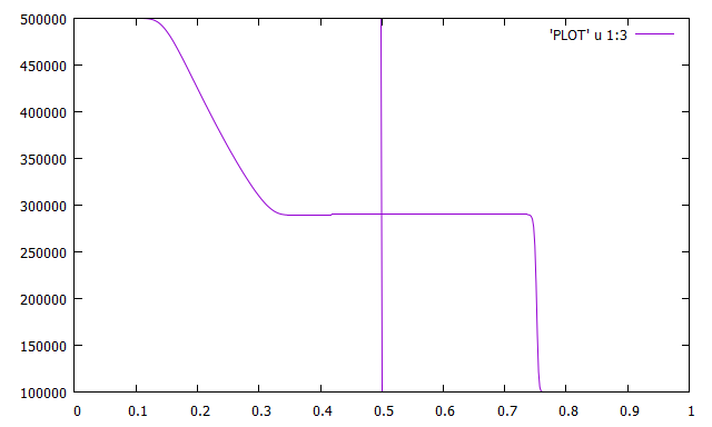
Figure 6.1 : Pressure solution vs x obtained after 250 timesteps with a mesh of 500 cells.
Hint
To plot with gnuplot software you can use the command in the gnuplot command windows:
- gnuplot> load ‘result.gnu’
(result.gnu is a file that contains gnuplot commands, you can also change these commands of this file!)
OR :
- gnuplot> plot ‘PLOT’ u 1:3